Time & Frequency Domain Signal Views
At Ham Radio School we really believe in the old adage that a picture is worth a thousand words. Visualization is often the key to understanding radio concepts. When it comes to visualizing signals, we use simplified visual models of signals that exhibit the important characteristics of signals, such as frequency, amplitude, and change over time. These visual models are not quite like real signals physically, but they provide us tools for thinking about signals in a simpler way.
Signals: Before we jump into our examination of signal graphical representations, let's consider what is meant by a signal. We need to understand the thing we want to represent with a visual model to ensure the visual model is not flawed in some fundamental way. One pertinent definition provided by Merriam-Webster for signal is: a detectable physical quantity or impulse (such as a voltage, current, or magnetic field strength) by which messages or information can be transmitted.
A signal may be a varying voltage or current within an electric circuit. The sounds of a radio operator's voice are converted by a microphone into AC voltages that represent moment-to-moment variation in voice frequencies and strengths. This band of dynamic audio frequencies is one type of baseband signal that is used to modulate a radio frequency carrier during the RF transmission process. These audio frequency signals are AC voltages, changing the direction of electrical force (voltage) in the microphone circuit from a few hundred to a few thousand times each second, creating commensurate surges of electrical current through the circuit that reverse direction at these same audio frequency rates. Physically, these signals are AC voltages and currents of a range of frequencies moving back-and-forth in the microphone circuit.
A radio transmitter merges the audio baseband signal with a radio frequency signal to place the audio information into radio frequency (RF) waveforms that can be efficiently transmitted through space as electromagnetic waves. While this modulation process is ongoing in the transmitter's circuits, the signals remain variations in electrical voltages and currents, although translated to much higher frequencies. These RF electrical signals energize an antenna, moving currents back and forth in the antenna's driven element. The result is the radiation of electromagnetic waves that mimic the frequency and strength variations of the electrical signals. The electrical signals that were voltage and current variations in a circuit are now electromagnetic (EM) wave signals traveling through space at the speed of light.
The upshot of this signal discussion is that signals may be generated at audio frequencies and at radio frequencies, and their physical form may be electrical or electromagnetic. A visual model must represent signals of either physical form, and the model should be able to depict signal frequency, strength, and variations in these over time.
Time & Frequency Domain Integrated Model: The two most common visual models of signals are the Time Domain View and the Frequency Domain View. These two signal depictions are closely related, as illustrated in the integrated 3D image of Figure 1.
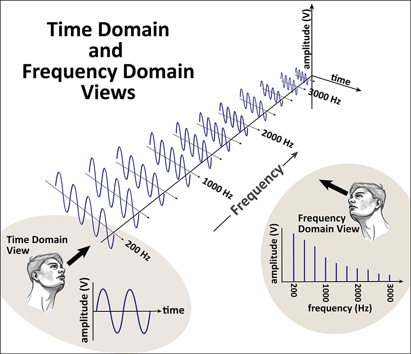
For this illustration, an audio band signal is depicted. The three axes of the Figure 1 illustration are:
Frequency Axis - (angled front-left to back-right.) Ranges from approximately 200 hertz to 3000 hertz in this illustration. Electrical signal oscillations are spread out across this continuous range. Only a subset of signal oscillations is depicted along this axis for simplification, but a continuous range of electrical oscillations may comprise a baseband audio signal such as a voice signal. The upward wave oscillations indicate voltage and current in an arbitrarily designated positive direction in a circuit, and the downward wave oscillations indicate voltage and current in the opposite "negative" direction.
Time Axis - (angled back-left to front-right.) Signal waveforms flow left-to-right along the time axis. The present instant of time is indicated by the intersection position of the three axes. Signal waveforms oscillate in positive-negative cycles as they flow along the time axis.
Amplitude Axis - (vertical axis.) The vertical extent of a signal waveform indicates the strength of the signal in terms of voltage or current. Signal oscillations in the positive (upward) direction and negative (downward) direction may vary over time, indicating changes in signal strength over time.
Notice that the signal waveforms may represent the positive-negative directions of voltage and current flow in a circuit, or they may represent the positive-negative oscillations of an EM wave as it propagates through free space. Normally, a signal will be depicted by either a Time Domain View or a Frequency Domain View, but not as an integrated 3D illustration as in Figure 1.
Time Domain View: The Time Domain View of a signal is captured from the perspective of the left-side observer of Figure 1 for which time becomes the horizontal axis. This observer views the model directly down the frequency axis to obtain a view as illustrated in the left-side inset graphic. Amplitude is depicted on the vertical axis. While more than one frequency can be overlaid onto a Time Domain View for comparisons, single frequency depictions in the time domain are more common. In this view, changes in frequency can be illustrated by compressed or expanded waveforms along the time axis. Amplitude changes over time can be depicted as variations in waveform height along the time axis.
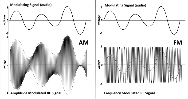
Figure 2 depicts Time Domain Views of both AM and FM modulation by an audio baseband signal. Amplitude is depicted as voltage variations, and the AM changes in amplitude of the RF signal mirror the audio waveform amplitude variations. The FM modulation depicts no amplitude changes of the RF signal, but rather frequency deviations driven by the amplitude of the audio signal. (The audio signal is replicated within the RF signal for illustration of this effect.)
Frequency Domain View: The Frequency Domain View of a signal is captured from the perspective of the right-side observer of Figure 1 for which frequency becomes the horizontal axis. This observer views the model directly down the time axis to obtain a view as illustrated in the right-side inset graphic. Again, amplitude is depicted on the vertical axis, and the range of frequencies in a signal is spread horizontally across the frequency axis. If the frequency domain were dynamic in time, the observer would see the spectrum of frequencies varying in amplitude over time. However, most Frequency Domain Views are static and depict only a single instant in time. When a continuous range of frequencies is depicted, the Frequency Domain View may contain filled or solid ranges across segments of frequency with amplitude variations depicted across the spectrum of frequency, as in Figure 3.
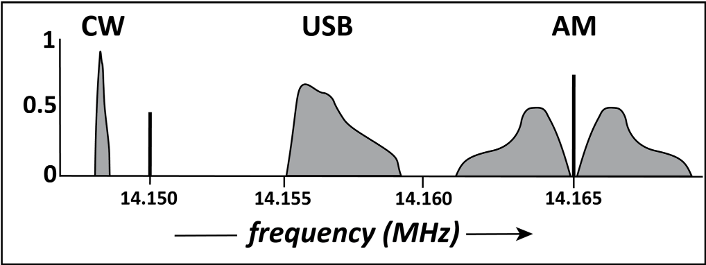
Figure 3 depicts a range of RF in the 20-meter band, with amplitude normalized to a 0-1 scale of voltage. A narrow spectrum CW signal is depicted below 14.150 MHz (left), and an upper sideband signal ranges from roughly 14.155-14.158 MHz (center). The two mirrored sidebands of an AM signal are centered on an RF carrier at 14.165 MHz.
Summary: Both Time Domain Views and Frequency Domain Views are used to represent signals of many types. The two views are linked, but usually depicted independently, depending on the purpose of the illustration. A Time Domain View depicts time on the horizontal axis, while a Frequency Domain View depicts frequency on the horizontal axis. Both of these types of signal model diagrams are utilized to illustrate radio principles throughout the Ham Radio School series of license preparation courses.