Power and Phase

The Technician and General license exams emphasize the concept of impedance matching to achieve maximum power transfer. This is often described as making sure the 50 Ω output of your transceiver drives a 50 Ω transmission line that connects to a 50 Ω antenna. In this article, we will go a little deeper to understand the role that phase plays in power transfer.
Figure 1 shows a resistive source and resistive load connected with the aim of transferring power from the source to the load. Most signal sources such as your transmitter have an internal resistance shown as RS in the figure. The load resistance, RL might represent the antenna or dummy load. The maximum power transfer principle can be stated as: “Maximum power is transferred when the internal resistance of the source equals the resistance of the load, when the external resistance can be varied, and the internal resistance is constant."
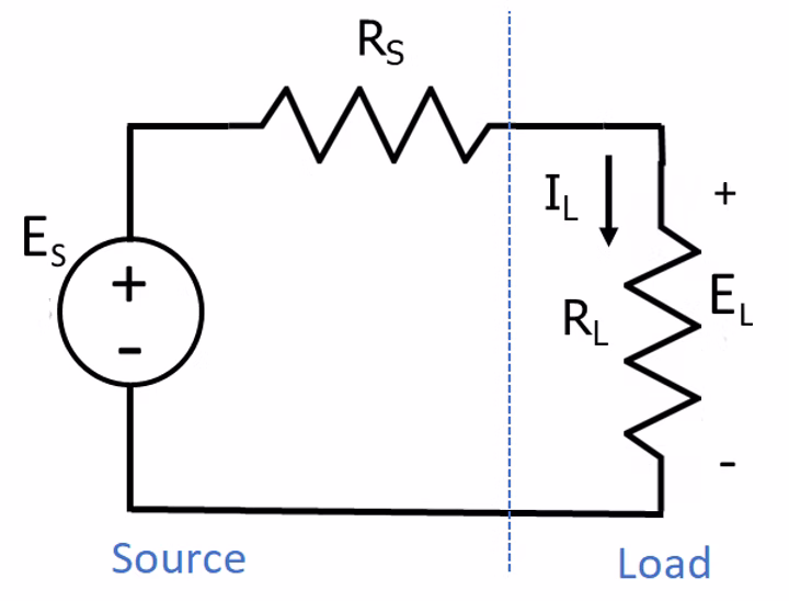
Figure 1. Circuit diagram showing a resistive source connected to a resistive load.
Figure 2 shows how the power to the load varies as a function of RL/RS. Power delivered to RL depends on both the current through the load and the voltage across the load. Large values of RL increase the voltage (EL) but starve the current (IL). Similarly, small values of RL increase the load current but diminish the load voltage. A bit of math can show that maximum power occurs when RL= RS.
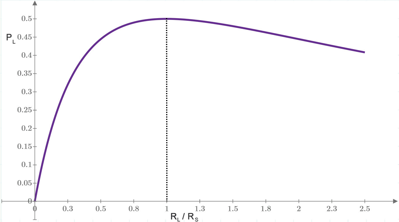
Figure 2. The plot of PL vs. RL/RS shows maximum power to the load when RL/RS =1.
Complex impedance Now consider the AC case where the impedances are complex, as shown in Figure 3. The source impedance is ZS = RS+ jXS and the load impedance is ZL= RL +jXL. The maximum power transfer occurs when ZLis the complex conjugate of ZS, which means RL= RSand XL = –XS. This is sometimes referred to as complex conjugate matching. As expected, if XS =0, the situation reduces back to the resistive case.
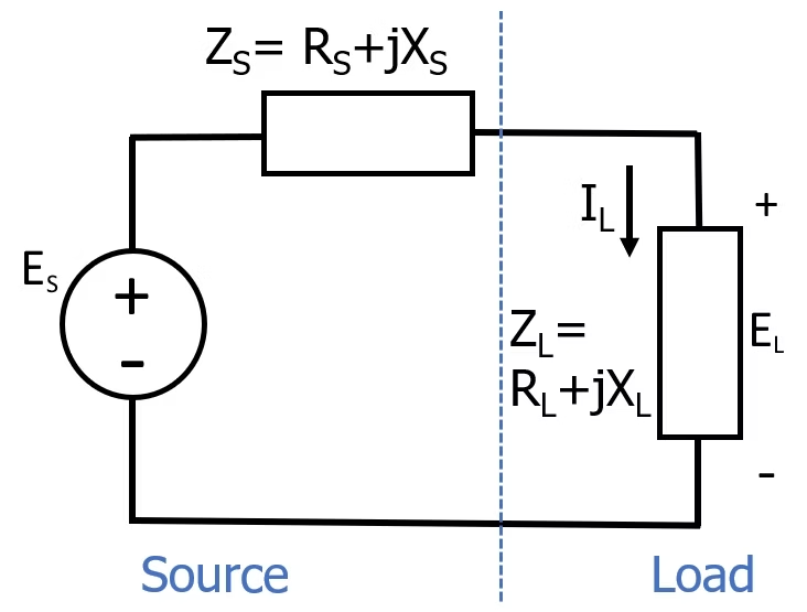
Figure 3. Circuit diagram showing a source connected to a load where both have complex impedances.
It's all about the phase Interestingly, when XL= –XS, the voltage source, ES sees a pure resistance (RS + RL), which means the current out of the voltage source is in phase with the voltage. This is not a coincidence; the phase between the voltage and current waveforms plays an important role in the average power in the load. Let's examine the time domain representations of instantaneous voltage, current, and power for a complex impedance.
Instantaneous power is given by
p (t )= e(t )i (t )
Assuming e(t ) and i (t ) are both sinusoids
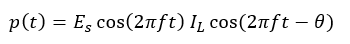
where ϴ is the phase difference between the voltage and current waveforms.
Figure 4 shows the time domain waveforms e(t ), i (t) and p(t ) for the case ϴ = 45°.
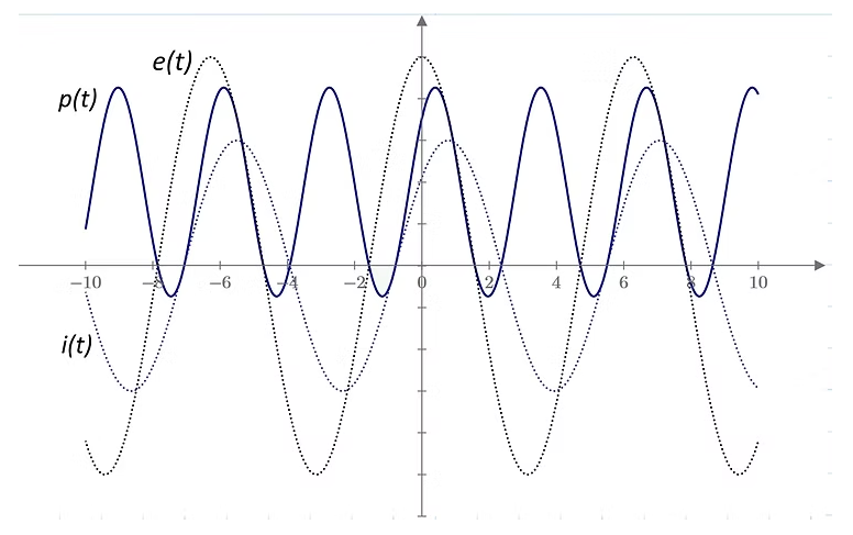
Figure 4. Plots of e (t ), i (t ) and p (t ) for the case ϴ = 45°.
We will skip the math, but the power equation can be reduced to:
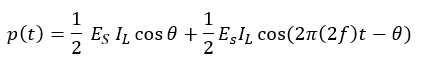
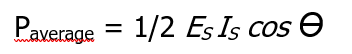
The expression for p (t ) is made up of a constant term and a cosine function at twice the original frequency. We are often interested in the average power in a waveform, which we can find by integrating p(t ) over one waveform period. The double frequency cosine term will average to zero, leaving only the constant term, so that
The plot of p(t ) in Figure 4 shows that the instantaneous power varies sinusoidally and even goes negative for part of the cycle. This is going to happen for all cases where ϴ does not equal zero. Also notice from the plot the average value of p(t ) is positive, indicating that power is delivered to the load.
Power engineers use the concepts of True Power and Apparent Power to quantify the effect that phase has on power. True Power represents the actual power transferred, which includes the effect of the phase between e and i , measured in units of Watts. Apparent Power is a more simplistic concept of just the raw current times the voltage, measured in units of Volt-Amps or VA to distinguish it from True Power.
Power engineers also use the concept of Power Factor (PF),
And it turns out that for sinusoidal waveforms, PF is equal to the cosine of the phase angle between the voltage and current waveforms.
Power Factor is a straightforward way to describe how much of the apparent power is being translated into useful (true) power. If ϴ = 0, then True Power and Apparent Power are the same and PF =1. When ϴ = ±90°, the True Power drops to zero and PF = 0. The example shown in Figure 4 with ϴ = 45°, PF = 0.707, which means that the True Power is 70% of the Apparent Power.
Wrap up We’ve reviewed the basics of maximum power transfer and the importance of phase relationships, tying it together with the power engineering concepts of power factor, true and apparent power. I intentionally ignored any discussion of transmission lines but these power transfer concepts have a lot in common with the usual transmission line concepts (standing wave ratio, return loss, reflection coefficient).
73-- Bob KØNR